Участник:АРыбников/Песочница

Априорная теория всего

физика

монография

Песочница

Автор:

Александр Рыбников

• Теория всего не от мира сего

Дата написания:

24 сентября 2023 года

Язык оригинала:

русский

Оригинал:

Теория всего не от мира сего

Предмет:

Решётчатая модель пространства-времени

https://proza.ru/avtor/alrybn1946

	Behind it all is surely an idea so simple, so beautiful, that when we grasp it - in a decade, a century, or a millennium - we will all say to each other, how could it have been otherwise? How could we have been so stupid?
— John Archibald Wheeler

Definition

A theory of everything — a physical-mathematical theory, all known variants of which have been carefully examined and rejected, now looks completely unexpected and fundamentally different from all previous versions.

Now it is the a priori theory of everything. It is the most detailed self-realizing project of the Metaverse, up to stars as self-forming, self-functioning, and self-removing thermonuclear reactors. In essence, the a priori theory of everything is the primary term of this theory and creates a naturally unified basis for the interpretation of cosmology, which studies the properties and evolution of the Metaverse as a whole, which is inaccessible to humanity in space and time. Hence, such a theory has no prototypes or variants in principle, because it is itself the only prototype. It comes at once and completely from a brief source, which, due to the above, is not written in any common language.

The latter means that the content of the a priori theory of everything arises as a result of the interpretation of the axiom, formulated as a mathematical formula. Its interpretation in the silence of the ages was done by mathematicians and physicists.

No Big Bangs, hundreds of inflations or Sinai in flames, shrouded in thick smoke; trembling earth; thundering thunder; flashing lightning; and in the noise and bedlam, covering it, the voice of God, uttering commandments (Ex. 19:1 and following). Nothing like this ever happened and could not happen in principle. No popular version of the stable functioning of the Metaverse will ever be written because of the mathematical formula underlying it.

Therefore, the goal of the a priori theory of everything is to build as long as possible a mathematical chain of consequences from the original axiom, including the exposition of cosmology. Thus, the interpretation introduces the relationship of the a priori axiom with the consequences observed in practice, that is, translates the original mathematical concepts of the axiom into physical language. The need to accept the axiom of existence without proof follows only from an inductive consideration: any proof is forced to rely on some statements and the chain will be infinite if you require your proofs for each of them. Nevertheless, explicit experimental evidence at the level of space and time, fundamental interactions, and elementary particles exist and they ‘break the infinite’. Thanks to this, it is always possible and necessary to go beyond the edge, to accept the challenges of developing physics.

In the a priori theory of everything, the question of the truth of the axiom of existence was solved almost 300 years ago.

Chronicles of the A Priori Theory of Everything

Leonhard Euler

From a distance, everything looks different.

Therefore, it can be said that on May 16 (27), 1703, at the mouth of the Neva River, Saint Petersburg was founded for the very purpose of creating an a priori theory of everything. On this day, Tsar Peter I laid the foundation of the Peter and Paul Fortress on the city’s first structure, Hare Island. Internal transformations and military victories in the Great Northern War contributed to the transformation of Russia into an Empire, which was officially proclaimed on October 22 (November 2), 1721, when, at the request of the senators, Peter I assumed the titles of Emperor of All Russia and Father of the Fatherland. Just a few years later, by imperial decree on January 22 (February 2), 1724, the Academy of Sciences and Arts was established in Saint Petersburg.

Subsequently, an edict by Empress Catherine I on February 23 (March 6), 1725, invited scholars to the Russian Academy of Sciences and provided the necessary support for those wishing to travel to Russia. In the early winter of 1726, Leonhard Euler (born April 15, 1707, Basel, Switzerland – died September 7 (18), 1783, Saint Petersburg, Russian Empire) received news from Saint Petersburg: based on the recommendation of the Bernoulli brothers, he was invited to the position of adjunct in the rapidly growing capital of the new world empire. His work in Saint Petersburg was so fruitful that it caught the attention of Russophobes:

	In mathematics, it is customary to name a discovery after the second person who made it, otherwise, everything would have to be named after Euler
— a humorous folk rule.

In particular, Euler continued research on the connection between the constant $\pi$ as a symbol of implicit $\infty$ and the constant $\ e$ as a symbol of explicit $\infty$, where Euler’s number $\ e$ — one of the most important mathematical constants — can be expressed as follows: $$\begin{equation*}\boxed{\ e = \sum_{n=0}^{\infty} \frac{1}{n!}. }\end{equation*}$$

The investigation of this connection began in 1714 with the publication of Euler’s formula, which asserts that for any real number $\varphi$, the following equality holds:

The geometric interpretation of Euler’s formula

$$\begin{equation*} \boxed{\ e^{i\varphi}=\cos \left(\varphi\right) +i\sin \left(\varphi\right).}\end{equation*}$$ This formula establishes a profound link between exponential functions, trigonometry, and complex numbers. It unifies these seemingly distinct mathematical concepts and plays a fundamental role in various fields of mathematics and physics. From here, when $\varphi=\pi$, Euler’s identity emerges, connecting five fundamental mathematical constants: $$\begin{equation*} \boxed{\ e^{i\pi}+1=0. }\end{equation*}$$

This remarkable equation unites the exponential function $\ e$, the imaginary unit $\ i$, the transcendental number $\pi$, the additive identity $0$, and the multiplicative identity $1$. It stands as a testament to the elegance and interconnectedness of mathematical concepts.

As a result, he made a fundamental contribution to the a priori theory of everything: in 1729, Leonhard Euler calculated the so-called “nonelementary antiderivative” integral: $\begin{equation} \label{axiom} \boxed{\frac{1}{\sigma\sqrt{2\pi}}\int_{-\infty}^{\infty}\ e^{-\frac{1}{2}(\frac{x}{\sigma})^{2}}dx=1.}\end{equation}$ This integral plays a crucial role in probability theory, statistics, and various scientific fields. Euler’s work continues to shape mathematical and scientific research to this day. Please, remember forever that the integral of the normal distribution was specifically calculated by Euler!

It should be noted that the mathematical meaning of this integral was clarified in 1929, when Bruno de Finetti (born on June 13, 1906, in Innsbruck; died on July 20, 1985, in Rome) introduced the concept of an infinitely divisible distribution. Such a distribution describes a random variable that can be represented as an arbitrary number of independent and identically distributed summands.

This marked a complete departure from Gauss’s idea, who believed that his theory only considered a single quantity.

James Clerk Maxwell

The role of Maxwell in the history of physics is not fully understood due to the fact that his equations represent the terms of the first order in an expansion with respect to the fine-structure constant. Thus, Maxwell created the quantum theory of electromagnetic radiation, which was the first theory to describe electricity, magnetism and light as different manifestations of the same phenomenon.

The next part of the history of the a priori theory of everything is a purely mathematical introduction of displacement current into Maxwell’s equations. Or, in modern terms, the introduction of magnetic monopoles.

Perhaps this is the first work in the history of physics where Hegel’s well-known proposition was successfully realized.

	What is reasonable is real; that which is real is reasonable.
— Georg Wilhelm Friedrich Hegel, Elements of the Philosophy of Right

Let’s keep in mind that Maxwell, justifying the mathematical introduction of displacement current, wrote in the language of that time (today such a funny language continues to be used by all sorts of ether worshipers). However, as a result of the development of his theory, Maxwell changed his understanding and abandoned the ether in favor of the displacement current.

So, under the influence of Faraday’s and Thomson’s ideas, Maxwell came to the conclusion that magnetism has a vortex nature, and the electric current - translational. For a vivid description of electromagnetic effects, he created a new, purely naive, mechanical model, according to which rotating “molecular vortices” produce a magnetic field, while the smallest transfer “idle wheels” provide rotation of vortices in one direction. The translational movement of these transfer wheels (“particles of electricity”, in Maxwell’s terminology) ensures the formation of an electric current. At the same time, the magnetic field, directed along the axis of rotation of the vortices, turns out to be perpendicular to the direction of the current, which found expression in the “screw rule” justified by Maxwell.

Within the framework of this mechanical model, Maxwell was able not only to give an adequate visual illustration of the phenomenon of electromagnetic induction and the vortex nature of the field generated by the current, but also to introduce an effect symmetrical to Faraday’s: changes in the electric field (the so-called displacement current, created by shifting the transfer wheels, or associated molecular charges, under the action of the field) should lead to the emergence of a magnetic field. The displacement current directly led to the continuity equation for the electric charge, that is, to the idea of open currents (previously all currents were considered closed). Considerations of symmetry of equations in this, apparently, did not play any role. The famous physicist J. J. Thomson called the discovery of the displacement current “Maxwell’s greatest contribution to physics”. These results were set out in the article “On physical lines of force”, published in several parts in 1861-1862.

In the same article, Maxwell, moving on to considering the propagation of disturbances in his model, noted the similarity of the properties of his vortex medium and Fresnel’s light-bearing ether. This found expression in the practical coincidence of the speed of propagation of disturbances (the ratio of the electromagnetic and electrostatic units of electricity, defined by Weber and Rudolf Kohlrausch) and the speed of light, measured by Hippolyte Fizeau. Thus, Maxwell made a decisive step towards the construction of the electromagnetic theory of light:

	We can hardly refuse to conclude that light consists of transverse oscillations of the same medium that is the cause of electrical and magnetic phenomena.
— James Clerk Maxwell

However, this medium (ether) and its properties were not of primary interest to Maxwell, although he certainly shared the view of electromagnetism as a result of applying the laws of mechanics to the ether:

	Maxwell does not give a mechanical explanation of electricity and magnetism; he limits himself to proving the possibility of such an explanation.
— Henri Poincaré

In 1864, Maxwell published the article “A Dynamical Theory of the Electromagnetic Field,” in which he gave a more detailed formulation of his theory (the term “electromagnetic field” appeared here for the first time). In doing so, he discarded the crude mechanical model (such representations, according to the scientist, were introduced exclusively “as illustrative, not as explanatory”), leaving a purely mathematical formulation of the field equations (Maxwell’s equations), which for the first time were treated as a physically real system with a definite energy. In the same work, he effectively proposed the hypothesis of the existence of electromagnetic waves, although, following Faraday, he wrote only about magnetic waves (electromagnetic waves in the full sense of the word appeared in the 1868 article). The speed of these transverse waves, according to his equations, is equal to the speed of light, and thus the concept of the electromagnetic nature of light was finally formed. Moreover, in the same work, Maxwell applied his theory to the problem of the propagation of light in crystals, the dielectric or magnetic permeability of which depends on the direction, and in metals, obtaining a wave equation taking into account the conductivity of the material.

Thus, the most important contribution to the concept of the theory of everything was made by Maxwell in the work “On Physical Lines of Force,” consisting of four parts and published in 1861-1862, in which the necessity of introducing a fundamentally new concept of displacement current was shown. Generalizing Ampère’s law, Maxwell introduces the displacement current, probably to link currents and charges by the continuity equation, which was already known for other physical quantities. Therefore, in this article, the formulation of the complete system of electrodynamics equations was essentially completed. In the 1864 article “A Dynamical Theory of the Electromagnetic Field,” the previously formulated system of 20 equations for 20 unknowns was considered. In this article, Maxwell first formulated the concept of the electromagnetic field as a physical reality, having its own energy and finite propagation time, determining the delayed nature of electromagnetic interaction.

Some physicists opposed Maxwell’s theory (especially many objections were raised by the concept of displacement current). Helmholtz proposed the own theory, a compromise relative to the models of Weber and Maxwell, and entrusted his student Heinrich Hertz to conduct its experimental verification. However, Hertz’s experiments unequivocally confirmed the correctness of Maxwell.

Arnold Sommerfeld

The need to write this chapter is due to the fact that it marks the end of the period of spontaneous approaches to the a priori theory of everything and the beginning of its crystallization. In natural science, such moments mature regularly and scientists themselves overcome them more or less painlessly. It should be noted that the damned secret of physics does have Russian roots, as its creator was born and studied in the semi-exclave of the Kaliningrad region of Russia (like Alaska for the USA). In 1891, Arnold Sommerfeld defended his doctoral dissertation in Kaliningrad (then still Königsberg) and then settled in Munich in search of work.

In 1913, Sommerfeld became interested in the research of the Zeeman effect, which was being conducted by the famous spectroscopists Friedrich Paschen and Ernst Back, and attempted to theoretically describe the anomalous splitting of spectral lines based on the generalization of Lorentz’s classical theory. Quantum ideas were used only to calculate the intensities of the splitting components. In July 1913, the famous work of Niels Bohr was published, which contained a description of his atomic model, according to which an electron in an atom can rotate around the nucleus along so-called stationary orbits without emitting electromagnetic waves. Sommerfeld was well acquainted with this article, a copy of which he received from the author himself, but at first he was far from using its results, having a skeptical attitude towards atomic models as such. Nevertheless, already in the winter semester of 1914-1915, Sommerfeld read a course of lectures on Bohr’s theory, and around the same time, he had thoughts about the possibility of its generalization (including relativistic).

The need for a generalization of Bohr’s theory was associated with the lack of a description of more complex systems than hydrogen and hydrogen-like atoms. In addition, there were small deviations of the theory from experimental data (lines in the spectrum of hydrogen were not truly single), which also required explanation. In one of the reports of the Bavarian Academy of Sciences and in the second part of his large article "On the Quantum Theory of Spectral Lines" (Zur Quantentheorie der Spektrallinien, 1916), Sommerfeld presented a relativistic generalization of the problem of an electron moving around the nucleus along an elliptical orbit, and showed that the perihelion of the orbit in this case slowly precesses. Sommerfeld managed to obtain a formula for the total energy of the electron, which included an additional relativistic term, determining the dependence of energy levels on both quantum numbers separately. As a result, the spectral lines of a hydrogen-like atom should split, forming the so-called fine structure, and the dimensionless constant introduced by Sommerfeld, the fine structure constant $\alpha$ (FSC), determined the magnitude of this splitting. Precision measurements of the spectrum of ionized helium, conducted by Friedrich Paschen in the same year of 1916, confirmed Sommerfeld’s theoretical predictions.

The constant $\alpha$ in the SI system of units can be defined as follows: $$\begin{equation} \label{alpha} \boxed{\alpha=\frac{e^2}{\ 4 \pi \varepsilon_0 \hbar c}=\frac{e^2}{2 \varepsilon_0 h c}}\end{equation},$$ where e is the charge of an electron, ε₀ is the permittivity of free space, ħ is the reduced Planck constant and c is the speed of light.

The success in describing the fine structure was a testament in favor of both Bohr’s theory and the theory of relativity and was enthusiastically accepted by a number of leading scientists.

	Your spectral studies are among the most beautiful things I have experienced in physics. Thanks to them, Bohr’s idea becomes completely convincing.
— Einstein

In his Nobel lecture (1920), Planck compared Sommerfeld’s work with the theoretical prediction of the planet Neptune. However, some physicists (especially those anti-relativistically inclined) considered the results of the experimental verification of the theory unconvincing. A strict derivation of the fine structure formula was given by Paul Dirac in 1928 based on a consistent quantum-mechanical formalism, so it is often called the Sommerfeld-Dirac formula. This coincidence of results, obtained within the framework of Sommerfeld’s semi-classical method and with the help of Dirac’s rigorous analysis (taking into account spin!), was interpreted differently in the literature. Perhaps the reason for the coincidence lies in an error made by Sommerfeld and turned out to be very handy. Another explanation is that in Sommerfeld’s theory, the neglect of spin successfully compensated for the lack of a rigorous quantum-mechanical description. Such a detailed description of the vicissitudes of the appearance of the FSC is given because at this time the First World War was already in full swing - one of the two most powerful and most terrible armed conflicts in human history. After the end of the First World War, the development of all physics accelerated. First of all, this concerned the discovery of new fundamental interactions, which at first glance no longer had anything in common with Maxwell’s equations. Thus, the original goal was finally lost - the description based on Maxwell’s equations of both space and time itself, and all fundamental interactions, as well as the existence of fundamental elementary particles. Subsequently, in quantum electrodynamics, the fine structure constant $\alpha$ acquired the value of the interaction constant, characterizing the intensity of interaction between electric charges and photons.

Paul Dirac

The next important step towards creating a theory of everything was made by Dirac in 1931 in the article “Quantized Singularities in the Electromagnetic Field”, where he introduced the concept of a magnetic monopole, whose existence could explain the quantization of electric charge. Later, in 1948, he returned to this topic and developed a general theory of magnetic poles, considered as ends of unobservable strings. Since then, magnetic monopoles have firmly entered modern physics.

For the a priori theory of everything, the idea of the magnetic monopole introduced by Dirac is fundamentally important, and the relationship between the magnitudes of the magnetic and electric charge established in his article is: $$\begin{equation} \label{monopol} \boxed{\frac{q_{S}}{q_{e}}=\frac{q_{N}}{q_{p}}=\frac{1}{2\alpha},}\end{equation},$$ where $q_{S}$ and $q_{N}$ are the charges of the Dirac magnetic monopole, $q_{e}$ is the charge of the electron, and $q_{p}$ is the charge of the positron. Since the denominators contain the charges of the particle and antiparticle, it can be expected that the numerators also contain the charges of the particle and antiparticle!

From the perspective of the theory of everything, this idea has advanced physics so much that even Dirac himself could not fully appreciate its consequences. In fact, a similar situation occurred a few years earlier when Dirac predicted the positron and proposed the idea of the “Dirac sea”.

Unfortunately, the fundamentally incorrect idea of particle birth and annihilation attracted more attention than the correct idea of the magnetic monopole. It is unlikely that Dirac himself was fully responsible for it in the sense that energy can create the mass of any particle. However, Dirac did say something about the existence of ready positrons in the “Dirac sea”! Followers of the idea of particle birth and annihilation applied it directly to the vacuum, behind which the ether, rejected by Maxwell, clearly emerged!

Nevertheless, after the prediction of antiparticles and their successful experimental confirmation, finding a magnetic monopole was not as quick. For a trivial reason. No one understood the essence of the formula, which stated that the intensity of interaction of magnetic monopoles significantly exceeds the intensity of interaction of electric charges! This meant that no means available to experimenters could register a magnetic monopole.

Indeed, Dirac himself added fuel to the fire.

	It seems that one of the fundamental properties of nature is that the basic physical laws are described by a mathematical theory with such elegance and power that an extremely high level of mathematical thinking is required to understand it. You may ask: why is nature arranged this way? The only answer is that our modern knowledge shows that nature is apparently arranged in this way. We just have to agree with it. Describing this situation, one could say that God is a mathematician of a very high class, and in constructing the Universe, He used very complex mathematics.”
— P. A. M. DiracProperty "Цитата/Автор" (as page type) with input value "— P. A. M. Dirac[3]" contains invalid characters or is incomplete and therefore can cause unexpected results during a query or annotation process.

As a result, most physicists declared Dirac’s magnetic monopoles hypothetical particles.

Later, in 1948, he returned to this topic and developed it into a more general concept of a non-local particle considered as the ends of an unobservable “string” for displacement current. Since then, magnetic monopoles have firmly entered modern physics as current-carrying particles. As if both in one bottle.

Unfortunately, he did not unequivocally express this idea. Therefore, Dirac’s magnetic monopoles were developed into the idea of dyons (or diions) by J. Schwinger in 1969. Schwinger introduced the dyon as a particle representing an electrically charged magnetic monopole.

And thousands of physicists, trained exclusively for the nuclear project, began to produce very expensive and high-quality junk at a tremendous speed. In addition to electromagnetic and gravitational interactions, contrived ones appeared: the so-called weak and strong. To these non-existent interactions, non-existent particles were also invented. And this direction of physics ended with the big bang dummy, which has no more intellect than a big mac!

	$\mathrm{N}\!\!\mathrm{B}$ Unfortunately, Dirac himself did not explicitly state that the magnetic monopole he introduced is the carrier of the strongest interaction. Perhaps for him, it was so obvious that he did not dare to tell experimenters that “a magnetic monopole can only be observed with another magnetic monopole.” Accordingly, he did not present the trivial consequence of the strongest interaction — the formation of a crystal from its carriers. On the other hand, if Dirac had explicitly said this, physics could have done without the “strong interaction” of H. Yukawa, quarks, and much more.
— Aleksandr Rybnikov, author

Mathematical Foundations of Obtaining a Fine Structure Constant

	It's one of the greatest damn mysteries of physics: a magic number that comes to us with no understanding by man. You might say the "hand of God" wrote that number, and "we don't know how He pushed his pencil." We know what kind of a dance to do experimentally to measure this number very accurately, but we don't know what kind of dance to do on the computer to make this number come out, without putting it in secretly!
― Richard P. FeynmanProperty "Цитата/Автор" (as page type) with input value "― Richard P. Feynman[4]" contains invalid characters or is incomplete and therefore can cause unexpected results during a query or annotation process.

As always, the experimenters were against it. They were fishing in murky waters, trying to detect the heterogeneity of the fine-structure constant in time or space. As a result, the relevance of searching for a mathematical formulation of the FSC fell by the wayside.

Intensity of interactions

If we choose an object that participates in all fundamental interactions, then the values of the dimensionless constants of these interactions, found by the general rule, will show the relative intensity of these interactions. The proton is most often used as such an object at the level of elementary particles. The basic energy for comparing interactions is the electromagnetic energy of a photon, which is defined as: $$U_f= \frac{h c}{\lambda}.$$ The choice of photon energy is not random, as the wave representation, based on electromagnetic waves, lies at the heart of modern physics. With their help, all basic measurements are made — lengths, times, and including energy.

Spatial Hyperanalytic Function

Idea

It is known that there is a fundamental relationship between the analyticity of a function and the rate of decay of its Fourier coefficients.

The better the function, the faster its coefficients tend to zero, and vice versa. Power decay of Fourier coefficients is inherent in polynomials, and exponential decay is inherent in analytic functions. However, it turns out that the generating function for the FSC does not belong to the specified types of functions, as a distinctive feature of the mathematical equations of quantum mechanics is the presence in them of the symbol of Planck’s constant. Hence follows the possibility of the existence of hyperanalytic functions, for which the decay of Fourier coefficients corresponds to tetration.

In addition, it should be clarified that, unlike traditional physics, the a priori theory of everything unexpectedly considers two types of fundamental interactions: spatial and temporal.

Definition of Spatial Hyperanalytic Function (SHF)

	The integral itself $\left(\ref{axiom}\right)$ is useless since it is not taken. As is known, there is no chance to find the keys lost at night somewhere. They should be looked for exactly under the lamp. Spatial fundamental interactions are manifested in the decomposition of the spatial lattice function $\mathbb{R}\left(x\right)$. $$\boxed{\frac{1}{\sigma\sqrt{2\pi}}\int_{-\infty}^{\infty}e^{-\frac{1}{2}(\frac{x}{\sigma})^{2}}dx=\frac{1}{\sigma\sqrt{2\pi}}\int_{-\frac{L}{2}}^{\frac{L}{2}}\sum_{n=-\infty}^{\infty}e^{-\frac{1}{2}(\frac{x-nL}{\sigma})^{2}}dx=1.}$$ This is where Euler’s dream comes from: quantification of monotonic exponential functions turns them into oscillatory trigonometric functions: $$\begin{equation} \label{hiper} \boxed{\mathbb{R}(x)=\frac{1}{\sigma\sqrt{2\pi}}\sum_{n=-\infty}^{\infty}e^{-\frac{1}{2}(\frac{x-nL}{\sigma})^{2}}.} \end{equation}$$
— Aleksandr Rybnikov, author

Decomposition of SHF

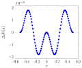
The graphs of the SHF and its components, presented in the gallery, clearly demonstrate that the decrease in Fourier coefficients for hyperanalytic functions corresponds to tetration.

• The graphs of the SHF and its components
• 

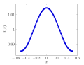
  SHF

• 

  First Difference of SHF

• 

  Second Difference of SHF

• 

  Third Difference of SHF

• 

  Fourth Difference of SHF

• 

  Fifth Difference of SHF

As mentioned earlier, the deviation of the function $\mathbb{R}\left(x\right)$ from one is of interest. From the SHF graph, it can be seen that the maximum value of SHF is reached when x=0: $$\mathbb{R}\left(0\right)=\mathbb{R}_{max}=\frac{1}{\sigma\sqrt{2\pi}}\sum_{n=-\infty}^{\infty}e^{-\frac{1}{2}\left(\frac{-n}{\sigma}\right)^{2}}.$$

The minimum value of the PRF is reached when x=1/2: $$\mathbb{R}\left(1/2\right)=\mathbb{R}_{min}=\frac{1}{\sigma\sqrt{2\pi}}\sum_{n=-\infty}^{\infty}e^{-\frac{1}{2}\left(\frac{1/2-n}{\sigma}\right)^{2}}.$$

	Let’s introduce the mathematical function of fine structure $\mathbb{\alpha}\left(\sigma\right)$ as the average relative value of the unevenness of the distribution of filling a unit segment by the function $e^{-\frac{1}{2}(\frac{x}{\sigma})^{2}}$, depending on $\sigma$: $$\begin{equation} \label{newtalpha} \boxed{\mathbb{\alpha}\left(\sigma\right)=\frac{1}{2}\frac{\mathbb{R}_{max}-\mathbb{R}_{min}}{\mathbb{R}_{max}+\mathbb{R}_{min}}.}\end{equation}$$
— Aleksandr Rybnikov, author

The choice of the name and designation of the parameter $\mathbb{\alpha}$ is due to the fact that $$\mathbb{\alpha}\left(0.4992619105929628\right)=\alpha.$$ Now everyone knows the solution to the cursed mystery of physics that has existed for more than a hundred years!

Since the distribution of filling a unit square with the function $e^{-\frac{1}{2}(\frac{x}{\sigma})^{2}}$ turns out to be above and below one, a deuce must be present in the definition, just as in formula $\left(\ref{alpha}\right)$. Thus, there are no other mathematical constants in formula $\left(\ref{alpha}\right)$.

The slight difference of $\sigma$ from the natural value of 0.5 will be explained later. Let $A_{0}$ is the constant term of the decomposition of SHF: $$A_{0}=\frac{\mathbb{R}_{max}+\mathbb{R}_{min}}{2}.$$ As a result of subtracting $A_{0}$ from $\mathbb{R}(x)$, we obtain the first difference.

Примечания

АРыбников